Tuesday, March 01, 2011

Learning data science skills

According to Hal Varian and just about everyone these days, the hot skills to have are some combination of programming, statistics, machine learning, and visualization. Here are a pile of resources that'll help you get some mad data science skills.

Programming

There seems to be a few main platforms widely used for data intensive programming. R, is a statistical environment that is to statisticians what MatLab is to engineers. It's a weird beast, but it's open source and very powerful, plus has a great community. Python also makes a strong showing, with the help of NumPy, SciPy and matplotlib. An intriguing new entry is the combination of the Lisp dialect Clojure and Incanter. All these tools mix numerical libraries with functional and scripting programming styles in varying proportions. You'll also want to look into Hadoop, to do your big data analytics map-reduce style in the cloud.

Statistics

  • John Verzani's Using R for Introductory Statistics, which I'm working my way through.
  • Machine Learning

  • Toby Segaran's Programming Collective Intelligence
  • The Elements of Statistical Learning: Data Mining, Inference, and Prediction
  • Bishop's Pattern Recognition and Machine Learning
  • Machine Learning, Tom Mitchell
  • Visualization

  • Tufte's books, especially The Visual Display of Quantitative Information
  • Processing, along with Ben Fry's book, Visualizing Data.
  • Jeffrey Heer's papers, especially Software Design Patterns for Information Visualization. Heer is one of the creators of several toolkits: Prefuse, Flare and Protovis.
  • 7 Classic Foundational Vis Papers and Seminal information visualization papers
  • Classes

    Starting on March 5 at the Hacker Dojo in Mountain View (CA), Mike Bowles and Patricia Hoffmann will present a course on Machine Learning where R will be the "lingua franca" for looking at homework problems, discussing them and comparing different solution approaches. The class will begin at the level of elementary probability and statistics and from that background survey a broad array of machine learning techniques including: Unsupervised Learning, Clustering Techniques, and Fault Detection.

    R courses from Statistics.com

    Feb 11:  Modeling in R (Sudha Purohit -- more details after the jump)
    Mar 4:  Introduction to R - Data Handling (Paul Murrell)
    Apr 15:  Programming in R (Hadley Wickham)
    Apr 29:  Graphics in R (Paul Murrell)
    May 20:  Introduction to R – Statistical Analysis (John Verzani)

    Data bootcamp (slides and code) from the Strata Conference. Tutorials covering a handful of example problems using R and python.

    • Plotting data on maps
    • Classifying emails
    • A classification problem in image analysis

    Cosma Shalizi at CMU teaches a class: Undergraduate Advanced Data Analysis.

    More resources

    Monday, February 21, 2011

    Using R for Introductory Statistics, Chapter 5, hypergeometric distribution

    This is a little digression from Chapter 5 of Using R for Introductory Statistics that led me to the hypergeometric distribution.

    Question 5.13 A sample of 100 people is drawn from a population of 600,000. If it is known that 40% of the population has a specific attribute, what is the probability that 35 or fewer in the sample have that attribute.

    I'm pretty sure that you're supposed to reason that 600,000 is sufficiently large that the draws from the population are close enough to independent. The answer is then computed like so:

    > pbinom(35,100,0.4)
    [1] 0.1794694
    

    Although this is close enough for practical purposes, the real way to answer this question is with the hypergeometric distribution.

    The hypergeometric distribution is a discrete probability distribution that describes the number of successes in a sequence of k draws from a finite population without replacement, just as the binomial distribution describes the number of successes for draws with replacement.

    The situation is usually described in terms of balls and urns. There are N balls in an urn, m white balls and n black balls. We draw k balls without replacement. X represents the number of white balls drawn.

    R gives us the function phyper(x, m, n, k, lower.tail = TRUE, log.p = FALSE), which does indeed show that our approximation was close enough.

    > phyper(35,240000,360000, 100)
    [1] 0.1794489
    

    Since we're down with OCD, let's explore a bit further. First, since our population is defined and not too huge, let's just try it empirically. First, create our population.

    > pop <- rep(c(0,1),c(360000, 240000))
    > length(pop)
    [1] 600000
    > mean(pop)
    [1] 0.4
    > sd(pop)
    [1] 0.4898984
    

    Next, generate a boatload of samples and see how many of them have 35 or fewer of the special members.

    > sums <- sapply(1:200000, function(x) { sum(sample(pop,100))})
    > sum(sums <= 35) / 200000
    [1] 0.17935
    

    Pretty close to our computed results. I thought I might be able to compute an answer using the central limit theorem, using the distribution of sample means, which should be approximately normal.

    > means <- sapply(1:2000, function(x) { mean(sample(pop,100))})
    > mean(means)
    [1] 0.40154
    > sd(means)
    [1] 0.0479998
    > curve(dnorm(x, 0.4, sd(pop)/sqrt(100)), 0.2, 0.6, col='blue')
    > lines(density(means), lty=2)
    

    Shouldn't I be able to compute how many of my samples will have 35 or fewer special members? This seems to be a ways off, but I don't know why. Maybe it's just the error due to approximating a discreet distribution with a continuous one?

    > pnorm(0.35, 0.4, sd(pop)/sqrt(100))
    [1] 0.1537173
    

    This fudge gets us closer, but still not as close as our initial approximation.

    > pnorm(0.355, 0.4, sd(pop)/sqrt(100))
    [1] 0.1791634
    

    If anyone knows what's up with this, that's what comments are for. Help me out.

    Notes on Using R for Introductory Statistics

    Chapters 1 and 2

    Chapter 3

    Chapter 4

    Chapter 5

    Sunday, February 13, 2011

    The Tiger Mom and A Clockwork Orange

    True disciple is doing what you want.

    A wise friend once told me that. Amy Chua, better known as the Tiger Mother, wrote about discipline (from a different point of view) in Why Chinese Mothers Are Superior.

    What Chinese parents understand is that nothing is fun until you're good at it. To get good at anything you have to work, and children on their own never want to work, which is why it is crucial to override their preferences. [...] Tenacious practice, practice, practice is crucial for excellence; rote repetition is underrated in America. Once a child starts to excel at something -- whether it's math, piano, pitching or ballet -- he or she gets praise, admiration and satisfaction. This builds confidence and makes the once not-fun activity fun. This in turn makes it easier for the parent to get the child to work even more.

    For what it's worth, Chua's book is apparently less strident and more nuanced than the WSJ article. Anyway, like her methods or not, I have a lot of sympathy for a parent trying to teach her kids about delayed gratification, that you can do difficult things if you try, and that hard work pays off.

    If it's true that mastering a complex skill takes 10,000 hours of practice, then the persistence to push through those hours is a fairly important lesson to learn early. Recent research has caused a reappraisal in how much talent arrises from innate genius versus how much is the product of effort, practice and persistence.

    What brought to mind my old friend's remark about disciple was Paul Buchheit's take: motivation can be either intrinsic or extrinsic. Amy Chua is teaching her kids to be extrinsically motivated, to respond to the praise and admiration of others. You do it because you are told to. You put your energy into chasing the approval of external authorities. In contrast, he describes intrinsic motivation like this:

    To the greatest extent possible, do whatever is most fun, interesting, and personally rewarding (and not evil).

    Follow your heart, as hippy moms tell their children. Buccheit says, "I'm kind of lazy, or maybe I lack will power or discipline or something. Either way, it's very difficult for me to do anything that I don't feel like doing." Sounds familiar. "The intrinsic path to success is to focus on being the person that you are, and put all of your energy and drive into being the best possible version of yourself."

    The difference between intrinsic and extrinsic motivation is easily recognized in the moral dimension. In A Clockwork Orange, Anthony Burgess imagines the transfer of aesthetic sense from creation to violence. Deprived of outlet, creativity turns destructive. The main thrust of the story is an examination of attempts to impose an external morality by force versus growing an internal morality.

    Paul Buccheit was the software developer that originated Google's gmail. For myself, and I'm sure lots of others, a key attraction to programming was the ability to create in a powerful medium without asking anyone's permission. The creative freedom, the feeling that the authorities hadn't (yet) figured out how to lock things down was incredibly inspiring.

    It's easy to see how that attraction to technology meshes with Daniel Pink's elements of motivationautonomy, mastery, and purpose. If you've got root and a compiler, you've got autonomy. And it's all about a pissing contest of mastery. (This might partially explain the gender ratio in the field.) And technology is rife with appeals to higher purpose, from the open-source movement to the digital media that helped fuel the revolutions in Tunisia and Egypt.

    The Tiger Mom demands mastery before autonomy, leaving purpose firmly in the hands of the parent. Buccheit puts autonomy first, trusting in a natural sense of direction to lead to mastery and purpose. In terms of Maslow's hierarchy of needs, Amy Chua has the "esteem" level covered, but stops short of the top level - intrinsic self-directed creativity.

    Some suggest that American society erects a border fence at the entry to the highest level. Well, nobody ever mentions why it's always drawn as a pyramid, but there's probably a reason. Not everyone gets to be at the top. Usually, that's the realm only of the elite.

    David Cain of Raptitude writes under the title How to Make Trillions of Dollars, that the fundamentals of being a self-directed person are these:

    Creativity. Curiosity. Resilience to distraction. Patience with others.

    Cain defines self-reliance as “an unswerving willingness to take responsibility for your life, regardless of who had a hand in making it the way it is”.

    Again, we're basically talking about the top levels of the pyramid. But, I like the addition of resilience to distraction. Discipline is a hard sell in a culture the promotes immediate gratification and nonstop indulgence. It's hard to hear your own voice over the clamor of consumer culture and expectations from family, boss and everyone else. Hearing it is nearly impossible while drowning in distractions like twitter and facebook. And here's something else to remember about online amusements:

    If you're not paying, you're not the customer; you're the product.

    At a recent data mining conference I saw rooms full of marketers ready to slice, dice and mash up your personal data to more precisely target advertising. Resisting this attack is an essential skill of modern life. A healthy cynicism is a necessary defense mechanism. Hearing yourself think is only going to get harder.

    The flawed idea implicit in consumer culture is what you consume is what you are. But, valuing consuming over creating or doing is inevitably a dead end. The reason I'm not so hot on the iPad is that it's a device for consuming. The old macs were (marketed as) tools for programmers, graphic artists, musicians and film-makers -- in other works doers, builders and creators.

    Purpose has to come from values. The recent travails of the financial sector show what happens when motivations or at least incentives become disconnected from morals and values.

    Of course, lots of technology has a purpose no higher than selling golf clubs on the internet. And technology, itself, can be a distraction. It's easy to get caught up in a rat race of the latest whizzy buzzword laden language, tool or application framework dujour. For years, I've had a half-joking theory that the true purpose of the internet is to absorb the excess productivity of mankind.

    Creative, conceptual work driven by autonomy, mastery and purpose pursued with uninterrupted concentration. That begins to answer the question, how do we get some motivation, apply it to something good and inspire the same in those around us, especially our ungrateful screaming offspring.

    You can argue one way or another about whether a 13 year old has the foresight to be intrinsically motivated. I certainly didn't have the wherewithal at that age to set a long term goal. And pushing intrinsic motivation on your kids sounds to me something like imposing democracy by force. I doesn't make that much sense.

    It takes determination to undertake exhausting frustrating efforts whose payoff is distant and uncertain. Most things that are worth doing are hard. The drive and courage to try anyway is what makes real progress possible. That doesn't come easily, and neither does the judgement necessary to gauge what is worth while against the scale of your own values.

    From my current position, I don't particularly want to lecture anyone on how to succeed in life. I respond negatively to coercion and can be a champion slacker, both of which were much to the detriment of my academic career. Still, here it is:

    • Value creation over consumption.
    • Surround yourself with creators.
    • Do what you love, do it a lot, and do it hard.

    Tuesday, February 08, 2011

    Using R for Introductory Statistics, Chapter 5, Probability Distributions

    In Chapter 5 of Using R for Introductory Statistics we get a brief introduction to probability and, as part of that, a few common probability distributions. Specifically, the normal, binomial, exponential and lognormal distributions make an appearance.

    For each distribution, R provides four functions whose names start with the letters d, p, q or r followed by the family name of the distribution. For example, rnorm produces random numbers drawn from a normal distribution. The letters stand for:

    ddensity/mass function
    pprobability (cumulative distribution function) P(X <= x)
    qquantiles, given q, the smallest x such that P(X <= x) > q
    rrandom number generation

    Normal

    The Gaussian or normal distribution has a prominent place due to the central limit theorem. It is widely used to model natural phenomena like variations in height or weight as well as noise and error. The 68-95-99.7 rule says:

    • 68% of the data falls within 1 standard deviation of the mean
    • 95% of the data falls within 2 standard deviations of the mean
    • 99.7% of the data falls within 3 standard deviations of the mean

    To plot a normal distribution, define some points x, and use dnorm to generate the density at those points.

    x <- seq(-3,3,0.1)
    plot(x=x, y=dnorm(x, mean=0, sd=1), type='l')
    

    Binomial

    A Bernoulli trial is an experiment which can have one of two possible outcomes. Independent repeated Bernoulli trials give rise to the Binomial distribution, which is the probability distribution of the number of successes in n independent Bernoulli trials. Although the binomial distribution is discrete, in the limit as n gets larger, it approaches the normal distribution.

    x <- seq(0,20,1)
    plot(x=x, y=dbinom(x,20,0.5))
    

    Uniform

    A Uniform distribution just says that all allowable values are equally likely, which comes up in dice or cards. Uniform distributions come in either continuous or discrete flavors.

    Log-normal

    The log-normal distribution is a probability distribution of a random variable whose logarithm is normally distributed. If X is a random variable with a normal distribution, then Y = exp(X) has a log-normal distribution. Analogously to the central limit theorem, the product of many independent random variables multiplied together tends toward a lognormal distribution. It can be used to model continuous random quantities whose distribution is skewed and non-negative, for example income or survival.

    samples <- rlnorm(100, meanlog=0, sdlog=1)
    par(fig=c(0,1,0,0.35))
    boxplot(samples, horizontal=T, bty="n", xlab="log-normal distribution")
    par(fig=c(0,1,0.25,1), new=T)
    s <- seq(0,max(samples),0.1)
    d <- dlnorm(s, meanlog=0, sdlog=1)
    hist(samples, prob=T, main="", col=gray(0.9), ylim=c(0,max(d)))
    lines(density(samples), lty=2)
    curve(dlnorm(x, meanlog=0, sdlog=1), lwd=2, add=T)
    rug(samples)
    

    Exponential

    The exponential distribution is used to model the time interval between successive random events such as time between failures arising from constant failure rates. The following plot is generated by essentially the same code as above.

    More on probability distributions

    More Using R for Introductory Statistics

    Tuesday, February 01, 2011

    Annotated source code

    We programmers are told that reading code is a good idea. It may be good for you, but it's hard work. Jeremy Ashkenas has come up with a simple tool that makes it easier: docco. Ashkenas is also behind underscore.js and coffeescript, a dialect of javascript in which docco is written.

    Interesting ways to mix prose and code have appealed to me ever since I first discovered Mathematica's live notebook, which lets you author documents that combine executable source code, typeset text and interactive graphics. For those who remember the early 90's chiefly for their potty training, running Mathematica on the Next pizza boxes was like a trip to the future. Combining the quick cycles of a Read-evaluate-print-loop with complete word processing and mathematical typesetting encourages you to keep lovely notes on your thinking and trials and errors.

    Along the same lines, there's Sweave for R and sage for Python.

    Likewise, one of the great innovations of Java was Javadoc. Javadoc doesn't get nearly enough credit for the success of Java as a language. It made powerful API's like the collections classes a snap and even helped navigate the byzantine complexities of Swing and AWT.

    These days, automated documentation is expected for any language. Nice examples are: RubyDoc, scaladoc, Haddock (for Haskell). Doxygen works with a number of languages. Python has pydoc, but in practice seems to rely more on the library reference. Anyway, there are a bunch, and if your favorite language doesn't have one, start coding now.

    The grand-daddy of these ideas is Donald Knuth's literate programming.

    I believe that the time is ripe for significantly better documentation of programs, and that we can best achieve this by considering programs to be works of literature. Hence, my title: "Literate Programming."

    Let us change our traditional attitude to the construction of programs: Instead of imagining that our main task is to instruct a computer what to do, let us concentrate rather on explaining to human beings what we want a computer to do.

    The practitioner of literate programming can be regarded as an essayist, whose main concern is with exposition and excellence of style. Such an author, with thesaurus in hand, chooses the names of variables carefully and explains what each variable means. He or she strives for a program that is comprehensible because its concepts have been introduced in an order that is best for human understanding, using a mixture of formal and informal methods that reinforce each other.

    Indeed, Ashkenas references Knuth, calling docco "quick-and-dirty, hundred-line-long, literate-programming".

    This goodness needs to come to more language. There's a ruby port called rocco by Ryan Tomayko. And for Clojure there's marginalia.

    I love the quick-and-dirty aspect and that will be the key to encouraging programmers to do more documentation that looks like this. I hope they build docco, or something like it, into github. Maybe one day there will be a Norton's anthology of annotated source code.

    Vaguely related

    Sunday, January 23, 2011

    Using R for Introductory Statistics, Chapter 5

    Any good stats book has to cover a bit of basic probability. That's the purpose of Chapter 5 of Using R for Introductory Statistics, starting with a few definitions:

    Random variable
    A random number drawn from a population. A random variable is a variable for which we define a range of possible values and a probability distribution. The probability distribution specifies the probability that the variable assumes any value in its range.

    The range of a discrete random variable is a finite list of values. For any value k in the range, 0 ≤ P(X=k) ≤ 1. The sum over all values k in the range is 1.

    R sample function implements these definitions. For example, let's ask R to create a six-sided die for us.

    p.die <- rep(1/6,6)
    sum(p.die)
    

    Now, let's roll it 10 times.

    die <- 1:6
    sample(die, size=10, prob=p.die, replace=T)
    

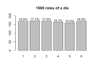
    Now, let's roll 1000 dice and plot the results.

    s <- table(sample(die, size=1000, prob=p.die, replace=T))
    lbls = sprintf("%0.1f%%", s/sum(s)*100)
    barX <- barplot(s, ylim=c(0,200))
    text(x=barX, y=s+10, label=lbls)
    
    Expected value
    Expected value (or population mean) of a discrete random variable X is the weighted average of the values in the range of X.

    In the case of our six-sided die, the expected value is 3.5, computed like so:

    sum(die*p.die)

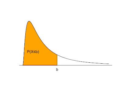
    Things change a bit when we move from discrete to continuous random variables. A continuous random variable is described by a probability density function. If f(x) is the probability density of a random variable X, P(X≤b) is the area under f(x) and to the left of b. The total area under f(x) = 1. f(x) ≥ 0 for all possible values of X. P(X>b) = 1 - P(X≤b). The expected value is the balance point where exactly half of the total area under f(x) is to the right and half is to the left.

    A random sample is a sequence of independent identically distributed random variables. A value derived from a random sample, such as sample mean, sample standard deviation, etc. is called a statistic. When we compute statistics of samples, our hope is that the sample statistic is not too far off from the equivalent measurement of the whole population.

    The interesting thing is that derived statistics are also random variables. If we role our die several times, we have taken a random sample of size n. That sample can be summarized by computing its mean, denoted by X bar.

    The sample mean is, itself, a random variable with its own distribution. So, let's take a look at that distribution. Because we'll use it later, let's define a function that generates a bunch of samples of size n and computes their means. It returns a vector of sample means.

    generate.sample.means <- function(n) {
      sample.means <- numeric()
      for (i in 1:1000) { 
        sample.means <- append(sample.means, sum(sample(die, size=n, prob=p.die, replace=T))/n)
      }
      return (sample.means)
    }
    
    sample.means <- generate.sample.means(100)
    plot(density(sample.means), main="Distribution of sample means",xlab="sample mean", col="orange")
    

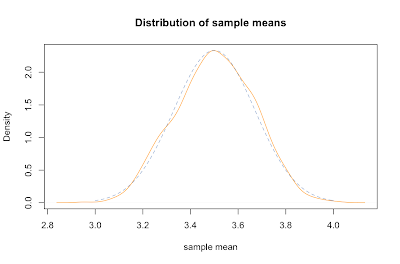
    Not coincidentally, it fits pretty closely to a normal distribution (dashed blue line). It's mean is about the same as the parent population, namely right around 3.5. The standard deviation of the sample means can be derived by dividing the standard deviation of the parent population by the square root of the sample size: σ / √ n.

    Let's compare the mean and sd of our sample with predicted values. We compute the standard deviation of our parent population of die rolls by squaring the deviation from the mean for each possible value and averaging that. Dividing that by the square root of our sample size gives the predicted sd of our sample means, about 0.17, which is about spot on with the actual sd.

    > mean(sample.means)
    [1] 3.49002
    > sd(sample.means)
    [1] 0.1704918
    > sqrt(sum( (1:6-3.5)^2 ) / 6) / sqrt(100)
    [1] 0.1707825
    

    To overlay the normal distribution on the plot above, we used R's dnorm function like this:

    x = seq(3,4,0.01)
    lines(x=x,y=dnorm(x,mean=3.5,sd=0.1707825), col=rgb(0x33,0x66,0xAA,0x90,maxColorValue=255), type="l", lty=2)
    

    Inspection of the formula for the standard deviation of sample means supports our common sense intuition that a bigger sample will more likely reflect the whole population. In particular, as the size of our sample goes up, our estimated mean is more likely to be closer to the parent population mean. This idea is known as the law of large numbers. We can show that it works by creating similar plots with increasing n.

    sample.means <- generate.sample.means(100)
    plot(density(sample.means), main="Distribution of sample means", xlab="sample mean", col="yellow", xlim=c(3.2,3.8), ylim=c(0,8))
    sample.means <- generate.sample.means(500)
    lines(density(sample.means), col="orange")
    sample.means <- generate.sample.means(1000)
    lines(density(sample.means), col="red")
    legend(3.6,7,c("n=100","n=500","n=1000"), fill=c("yellow", "orange", "red"))
    

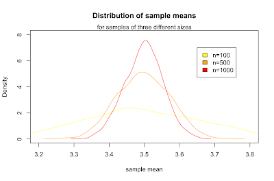
    What we've just discovered is the central limit theorem, which states that for any parent population with mean μ and standard deviation σ, the sampling distribution for large n is a normal distribution with mean μ and standard deviation σ / √ n. Putting that in terms of the standard normal distribution Z gives:

    It's a little surprising that the normal distribution arises out of a means of samples from a discrete uniform distribution. More surprisingly, samples from any parent distribution give rise to the normal distribution in exactly the same way. Next, we'll look at several widely used families of distributions and R's functions for working with them.

    Notes

    The graph above shaded in orange serving as an example probability density function is produced with the following R code:

    plot(x=c(seq(0,5,0.01)), y=c(dlnorm(x=seq(0,5,0.01),meanlog=0,sdlog=1)), type="l", xlab='', ylab='', yaxt="n", xaxt="n", bty="n")
    polygon(x=c(seq(0,2,0.01),2), y=c(dlnorm(x=seq(0,2,0.01),meanlog=0,sdlog=1),0), col="orange")
    mtext('b', at=c(2), side=1)
    text(0.6,0.2,"P(X≤b)")
    abline(c(0,0),c(0,5))
    

    More Using R for Introductory Statistics

    Sunday, January 09, 2011

    Using R for Introductory Statistics, Chapter 4, Model Formulae

    Several R functions take model formulae as parameters. Model formulae are symbolic expressions. They define a relationship between variables rather than an arithmetic expression to be evaluated immediately. Model formulae are defined with the tilde operator. A simple model formula looks like this:

    response ~ predictor

    Functions that accept formulae typically also take a data argument to specify a data frame in which to look up model variables and a subset argument to select certain rows in the data frame.

    We've already seen model formula used for simple linear regression and with plot and boxplot, to show that American cars are heavy gas guzzlers. Two common uses of formula are:

    • y ~ x where x and y are numeric
    • x ~ f where x is numeric and f is a factor

    The Lattice graphics package can accept more complicated model formulas of this form:

    response ~ predictor | condition

    We'll try this out with a dataset called kid.weights from the UsingR package. We get age, weight, height and gender for 250 kids ranging from 3 month to 12 years old.

    library(UsingR)
    library(lattice)
    dim(kid.weights)
    [1] 250   4
    

    We expect weight and height to be related, but we're wondering if this relationship changes over time as kids grow. Often, when we want to condition on a quantitative variable (like age), we turn it into a categorical variable by binning. Here, we'll create 4 bins by taking age in 3 year intervals.

    age.classes = cut(kid.weights$age/12, 3*(0:4))
    unique(age.classes)
    [1] (3,6]  (6,9]  (9,12] (0,3] 
    Levels: (0,3] (3,6] (6,9] (9,12]
    

    With age as a factor, we can express our question as the model formula:

    height ~ weight | age.classes

    The lattice graphics function xyplot accepts this kind of formula and draws a panel for each level of the conditioning variable. The panels contain scatterplots of the response and predictor, in this case height and weight, divided into subsets by the conditioning variable. The book shows a little trick that let's us customize xyplot, adding a regression line to each scatterplots.

    plot.regression = function(x,y) {
      panel.xyplot(x,y)
      panel.abline(lm(y~x))
    }
    

    We pass the helper function plot.regression as a custom panel function in xyplot.

    xyplot( height ~ weight | age.classes, data=kid.weights, panel=plot.regression)
    

    There's quite a bit more to model formulae, but that's all I've figured out so far.

    More on formulae