Sunday, December 27, 2009

SQL group by in R

The R ProjectThe R statistical computing environment is awesome, but weird. How to do database operations in R is a common source of questions. The other day I was looking for an equivalent to SQL group by for R data frames. You need this to compute summary statistics on subsets of a data set divided up by some categorical variable. It turns out there are several ways to get the same effect, some more limited than others.

The best answer seems to be plyr. It automates the The split-apply-combine strategy for data analysis you'd use otherwise. The ddply splits a data frame into subset data frames, performs some function on the subsets, and returns the results as a recombined data frame.

Here's a few links: A Fast Intro to Plyr for R, Block-processing a data frame with plyr and Split, apply, and combine in R using PLYR.

This paper is worth reading. It introduces the library and also gives you a nice framework (split-apply-combine) for thinking about a whole class of data-munging problems. A coworker (thanks, Gustavo) pointed out that this is a lot like Google's MapReduce.

Some commands that get you part of the way there are: split, by, tapply (nicely explained here), aggregate. The R wiki has an entry on Performing calculations within sub-sets of a data-frame that uses the reshape library. You could always use sqldf or RSQLite. Several options are discussed here. You can cobble up a fully general process using split, some form of sapply, and unsplit. But, that's what plyr does automatically.

Side notes: While fooling around with this, I noticed that, for some crazy reason, split.data.frame splits matrices into nice subunits, but split has the ugly side-effect of reducing matrices to vectors. Also, Google has a style guide for R.

More R mini-tutorials:

Links

Sunday, December 20, 2009

Layered architecture for a Java application

This is a template for an application architecture that came out of my genome browser project. This Java/Swing desktop application aspires to be very flexible - implementing new visualizations and accommodating task-specific components when necessary. I'm not sure how well I did at this goal, so don't take this as here's-what-you-should-do, just here's-what-one-poor-schmuck-did.

The Application object holds application scope state, and binds components together, performing dependency injection where necessary. The entry point is myapp.Main, which configures Options using command-line arguments and starts the application. The application manages a concurrent event dispatch queue.

Components communicate with each other by events placed on the event queue and have access to an application API. Like in Swing, component code may run in the thread of the event dispatch, or, if it is long running, spin up its own thread. Components are responsible for managing their own threading and synchronization.

Layering, in this template, works something like this:

+--------+
|   UI   |
+--------+
+-----------------+ +----------------+
|   Application   | |   components   |
+-----------------+ +----------------+
+--------------+
|   services   |
+--------------+
+------------+ +----------+
|   domain   | |   util   |
+------------+ +----------+

Higher layers can depend on lower layers, while dependencies may not flow up. Utilities and domain model can have no internal dependencies and anything may depend on them. Services are things like file I/O, persistence, and maybe algorithms. The application exposes an API to components and will in turn implement that API in terms of components. I think this circular dependency doesn't bother me too much. If it did, the Application could have no dependencies on the components and the components could have some organized dependency structure among themselves. The UI sits on top where nothing should depend on it.

Thursday, December 17, 2009

Joining data frames in R

The R ProjectWant to join two R data frames on a common key? Here's one way do a SQL database style join operation in R.

We start with a data frame describing probes on a microarray. The key is the probe_id and the rest of the information describes the location on the genome targeted by that probe.

> head(probes)
          probe_id sequence strand   start     end
1 mm_ex_fwd_000541      Chr      + 1192448 1192507
2 mm_ex_fwd_000542      Chr      + 1192453 1192512
3 mm_ex_fwd_000543      Chr      + 1192458 1192517
4 mm_ex_fwd_000544      Chr      + 1192463 1192522
5 mm_ex_fwd_000545      Chr      + 1192468 1192527
6 mm_ex_fwd_000546      Chr      + 1192473 1192532

> dim(probes)
[1] 241019      5

We also have a bunch of measurements in a numeric vector. For each probe (well, a few probes missing due to bad data) we have a value.

> head(value)
mm_fwd_000002 mm_fwd_000003 mm_fwd_000004 mm_fwd_000005 mm_fwd_000006 mm_fwd_000007 
   0.05294899    0.11979251    0.28160017    0.57284569    0.74402510    0.78644199 

> length(value)
[1] 241007

Let's join up these tables, er data frame and vector. We'll use the match function. Match returns a vector of positions of the (first) matches of its first argument in its second (or NA if there is no match). So, we're matching our values into our probes.

> joined = cbind(probes[match(names(value), probes$probe_id),], value)

> dim(joined)
[1] 241007      6

> head(joined)
          probe_id sequence strand start end         value
3695 mm_fwd_000002      Chr      +    15  74 0.05294899
3696 mm_fwd_000003      Chr      +    29  88 0.11979251
3697 mm_fwd_000004      Chr      +    43 102 0.28160017
3698 mm_fwd_000005      Chr      +    57 116 0.57284569
3699 mm_fwd_000006      Chr      +    71 130 0.74402510
3700 mm_fwd_000007      Chr      +    85 144 0.78644199

Merge is probably more similar to a database join.

Inner joinmerge(df1, df2, by="common_key_column")
Outer joinmerge(df1, df2, by="common_key_column", all=TRUE)
Left outermerge(df1, df2, by="common_key_column", all.x=TRUE)
Right outermerge(df1, df2, by="common_key_column", all.y=TRUE)

If we have two data frames, we can use merge. Let's convert our vector tp to a data frame and merge, getting the same result (in a different sort order).

> tp.df = data.frame(probe_id=names(tp), value=tp)

> head(tp.df)
                   probe_id      value
mm_fwd_000002 mm_fwd_000002 0.05294899
mm_fwd_000003 mm_fwd_000003 0.11979251
mm_fwd_000004 mm_fwd_000004 0.28160017
mm_fwd_000005 mm_fwd_000005 0.57284569
mm_fwd_000006 mm_fwd_000006 0.74402510
mm_fwd_000007 mm_fwd_000007 0.78644199

> m = merge(probes, tp.df, by="probe_id")

> dim(m)
[1] 241007      6

> head(mmm)
          probe_id sequence strand   start     end     value
1 mm_ex_fwd_000541      Chr      + 1192448 1192507 0.1354668
2 mm_ex_fwd_000542      Chr      + 1192453 1192512 0.1942794
3 mm_ex_fwd_000543      Chr      + 1192458 1192517 0.1924457
4 mm_ex_fwd_000544      Chr      + 1192463 1192522 0.2526351
5 mm_ex_fwd_000545      Chr      + 1192468 1192527 0.1922655
6 mm_ex_fwd_000546      Chr      + 1192473 1192532 0.2610747

There's a good discussion of merge on Stack Overflow, which includes right, left, inner and outer joins. Also the R wiki covers both match and merge. See also, the prior entry on select operations on R data frames.

Wednesday, December 16, 2009

Modern Information Management in Bioinformatics

Jon Udell talks bioinformatics with Randy Julian of Indigo BioSystems on the topic of flexible data repositories.

… without buying into all the hype around semantic web and so on, you would argue that a flexible schema makes more sense in a knowledge gathering or knowledge generation context than a fixed schema does.

His contention is that fixed schemas don't work for knowledge discovery, instead the right tools are flexible schemas and linked data. Also, it's not enough to represent experimental data in standard ways. We also need to describe the experimental design that provides the context for that data. To accomplish this use documents annotated with RDF style triples or XML plus (not-quite-free-text) descriptions built from controlled vocabulary. Use virtualization to archive complete data analysis environments for reproducability.

On the IndigoBio blog, there's a couple posts about interoperable data that make use of R and Cytoscape. Sounds like territory familiar to my current project/nemesis Gaggle.

The conversation then turns to the increasingly distributed nature of the drug industry and the IT challenges of strictly proscribed data sharing between highly paranoid competitors. The goal is to produce portable data assets with the ability to merge with any clients knowledge base -- mapping into the other's terms.

Related Links:

Thursday, December 10, 2009

Microformats

Jeff Atwood, who writes the well-known Coding Horror blog, took on the topic of Microformats recently. His misguided comments about the presumed hackiness of overloading CSS classes with semantic meaning (actually their intended purpose) had people quoting the HTML spec:

The class attribute, on the other hand, assigns one or more class names to an element; the element may be said to belong to these classes. A class name may be shared by several element instances. The class attribute has several roles in HTML:
  • As a style sheet selector (when an author wishes to assign style information to a set of elements).
  • For general purpose processing by user agents.

Browsers work great for navigation and presentation, but we can only really compute with structured data. Microformats combine the virtues of both.

There are at least a couple of ways in which the ability to script interaction with web applications comes in handy. For starters, microformats are a huge advance compared to screen-scraping. The fact that so many people suffered through the hideous ugliness of screen-scraping proves that there must be some utility to be had there.

Also, web-based data sources have a browser-based front-end and also often expose a web service. Microformats link these together. A user can find records of interest by searching in the browser, embedded microformats allow the automated construction of a web service call to retrieve the data in structured form.

Microformats aren't anywhere near the whole answer. But, the real question is how to do data integration at web scale using the web as a channel for structured data.

See also

Wednesday, December 09, 2009

Distilling Free-Form Natural Laws from Experimental Data

Eureqa software implements the symbolic regression technique described in this paper:

Schmidt M., Lipson H. (2009) "Distilling Free-Form Natural Laws from Experimental Data," Science, Vol. 324, no. 5923, pp. 81 - 85.

Monday, November 30, 2009

Design Patterns 15 years later

Design Patterns 15 Years Later: An Interview with Erich Gamma, Richard Helm, and Ralph Johnson was recently featured on Lambda the Ultimate.

Some say design patterns are just work-arounds for the defects of C++. The paper Essential Programming Paradigm argues that design patterns occur because the programming paradigm disallows certain run-time composition of dynamic and static code. The GoF authors confirm that their design patterns fit object-oriented languages, and arise specifically from experience with C++ and Smalltalk, so are tied to language of implementation. "Design patterns eventually emerge for any language. Design déjà-vu is language neutral." Different design patterns may be emerging for dynamic languages or for functional languages.

They discuss the development of more design patterns beyond the 23 examples chosen for the Design Patterns book. Eric Gamma suggest some sort of collective intelligence approach for editing design patterns and rating their importance and applicability. Sounds like a good idea. Some new patterns they mention as candidates for inclusion in a revised set are: Null Object, Type Object, Dependency Injection, and Extension Object/Interface. Their new (draft) categorization of design patterns looks like this:

They seem to have dropped several, some of which I won't miss. but why axe composite or observer? And bridge, maybe not the most useful in practise, but when I finally understood what they meant, I felt like I had accomplished something.

Design patterns links

Saturday, November 28, 2009

Leroy Hood on a career in science

ISBLeroy Hood, the founder of the Institute for Systems Biology, where I've worked for 3 years now, wrote up some career advice for scientists last year. It probably applies fairly well to any professional.

I leave students (and even some of my colleagues) with several pieces of advice. First, I stress the importance of a good cross-disciplinary education. Ideally, I suggest a double major with the two fields being orthogonal-say, biology with computer science or applied physics. Some argue that there is insufficient time to learn two fields deeply at the undergraduate level.

I argue that this is not true. If we realize that many undergraduate courses now taught are filled with details that are immediately forgotten after the course is finished, we must then learn to teach in an efficiently conceptual manner. As I noted above, as an undergraduate at Caltech I had Feynman for physics and Pauling for chemistry, and both provided striking examples of the power of conceptual teaching.

Second, I argue that students should grow accustomed to working together in teams: In the future, there will be many hard problems (like P4 medicine) that will require the focused integration of many different types of expertise.

Third, I suggest that students acquire an excellent background in mathematics and statistics and develop the ability to use various computational tools. Fourth, I argue that a scholar, academic, scientist, or engineer should have four major professional objectives: (a) scholarship, (b) education (teaching), (c) transferring knowledge to society, and (d ) playing a leadership role in the local community to help it become the place in which one would like one’s children and grandchildren to live.

Fifth, with regard to the scientific careers of many scientists-they can be described as bellshaped curves of success-they rise gradually to a career maximum and then slowly fall back toward the base line. To circumvent this fate, I propose a simple solution: a major change in career focus every 10 or so years. By learning a new field and overcoming the attendant insecurities that come from learning new areas, one can reset the career clock. Moreover, with a different point of view and prior experience, one can make fundamental new contributions to the new field by thinking outside the box. Then the new career curve can be a joined series of the upsides of the bellshaped curve, each reinvigorated by the ten-year changes.

Finally, science is all about being surrounded by wonderful colleagues and having fun with them, so I recommend choosing one’s science, environment, and colleagues carefully. I end this discussion with what I stressed at the beginning-I am so fortunate to have been surrounded by outstanding colleagues who loved science and engineering. Science for each of us is a journey with no fixed end goal. Rather, our goals are continually being redefined.

ISB recently topped 300 employees and, as of early 2009, had a budget of $55 million. Dr. Hood turned 70 in 2008.

Monday, November 09, 2009

Computational representation of biological systems

Computational representation of biological systems by Zach Frazier, Jason McDermott, Michal Guerquin, Ram Samudrala is a book chapter in Springer's Computational Systems Biology. It introduces basic data warehousing concepts along with a data warehousing effort targeted at biology called Bioverse.

They contrast data warehousing with online transaction processing. OLTP entails frequent concurrent updates. Updates traditionally look like bank machine operations or travel reservations. Data warehousing, in contrast, typically updates only occasionally in an additive way as new data arrives or annotations are added. The star schema, which supports efficient subsetting and computing of aggregates (min, max, sum, count, average), centers on a table of atomic data elements called facts surrounded by related tables holding different types of search criteria called dimensions.

Bioverse nicely illustrates several of the main problems challenges with data warehousing. First, it's data (54 organisms) appears to have been last updated in 2005. Also, we must choose at what granularity to create the fact table based on the questions we expect to ask, but questions come at many scales.

Hierarchical data occurs throughout the Bioverse. Representation of these structures is particularly difficult in relational databases.

They go on to cite a method for supporting efficient hierarchical queries from Kimball, R., Ross, M., (2002). The Data Warehouse Toolkit: The Complete Guide to Dimensional Modeling.

In addition to hierarchies, graphs and networks are common structures in biological systems including protein­protein interaction networks, biochemical pathways, and others. However, the techniques outlined for trees and directed acyclic graphs are no longer appropriate for graphs. Answering any more than very basic graph queries is hard in relational databases.

So, with all these drawbacks, you have to wonder whether the relational database is a good basis for data mining applications. Especially with the prevalence of networks in biological data. I'm a lot more intrigued by ideas along the lines of NoSQL schema-less databases, Dynamic fusion of web data and the web as a channel for structured data.

Friday, November 06, 2009

The Stories Networks Tell

Dr. Carl Bergstrom gave a very cool lecture on “The Stories Networks Tell” at UW a week or two ago. Eigenfactor applies network analysis methods to mapping the citation structure of academic journals. He has a nice method of discovering modularity in networks using random walks. There are some nice flash interactive graphics on his lab's website. It's cool that he's published on economics, evolution, infectious disease, and information theory. On the theme of biology and economics:

Tuesday, November 03, 2009

Elements of Programming

Don't you hate it when someone reads the first chapter of a book and then decides they're qualified to review it? So do I. But based on the first chapter, Elements of Programming by Alexander Stepanov, Paul McJones is something I might want to come back to, so here's my reminder to myself.

Stepanov is the guy behind the C++ Standard Template Library (STL), an advocate of generic programming and a critic of OOP. (papers here)

The authors have done for C++ something that is more commonly done for the functional languages, which is to put the language on a formal mathematical basis. Their central insight is the parallel between algorithms and data structures and algebraic structures. Abstract algebraic structures consist of one or more sets and one or more operations on those sets.

The formalism introduced in the book is based on objects with mutable state "computers with memory constitute the only available realization of a universal computing device". They seem to value that C++ is "faithful to the underlying machine". I wonder how this formalism will hold up to parallel computation, in contrast to the immutability and statelessness that seem popular in these increasingly parallel days. I also wonder about the comparison between this formalism and the lambda calculus.

They define a notion called regularity. A regular function is a pure side-effect-free function (If I'm reading right). Procedures and types can also be regular. A regular type is required to implement operation for equality, assignment, destructor, default constructor, copy constructor, total ordering, and underlying type. A concept is a minimal set of requirements a data type must satisfy for an algorithm to be applicable. Algorithms can then be implemented in terms of concepts rather than concrete data types. (I think?) Concepts can have semantic requirement like linear time complexity for a given operation, bringing efficiency into the mix.

Whether one likes this book will be strongly influenced by how well one likes generic programming in C++. And maybe whether one wants one's theory sullied by implementation details. I like the idea that generic programming can be something more than making a type checker happy -- more than the type-safe collections of Java's puny generics. And who would have thought you could extract a pretty mathematical theory from the warty ugster known as C++?

A reviewer on Amazon suggests a related Google Tech Talk "A Possible Future of Software Development" by Sean Parent.

Saturday, September 26, 2009

Color for Programmers

Good visual design matters in software and in visualization. Sadly, most of us engineers are lucky to put on two matching socks in the morning, much less master the subtle art of graphic design. Fortunately, there are resources for the rest of us.

...or just google for color scheme

Saturday, September 05, 2009

Closure

I've heard nice things about Clojure. Stuart Halloway has a book (Programming Clojure) out through the Pragmatic Programmers. The book grew out of Stuart's Java.next series of articles. There's also a podcast.

Clojure, like Scala, is functional programming for the JVM. Scala (which I fooled around with a little) descends from the ML/Caml/O-caml family of languages with an emphasis on pattern matching and static typing with type inference. Clojure is a dynamic Ruby-influenced dialect of Lisp specifically targeted to the JVM (hence the j). Yet another programming language on the digithead's cool-technology-I-want-to-play-with list.

Update

Wednesday, August 26, 2009

Using R and Bioconductor for sequence analysis

Here's another quick R vignette, in case I pick this up later and need to remind myself where I got stuck. I was trying to use R for a bit of basic sequence analysis, with mixed results.

First, install the BSgenome package, which is part of Bioconductor. Get GeneR while you're at it.

> source("http://bioconductor.org/biocLite.R")
> biocLite("BSgenome")
> biocLite("GeneR")

Follow the instructions in the document How to forge a BSgenome data package. You'll need to get fasta files from somewhere such as NCBI's Entrez Genome. Another nice data source is Regulatory Sequence Analysis Tools.

I created a BSgenome package for our favorite model organism Halobacterium salinarum NRC-1, which I named halo for short. Now, I can ask what sequences make up the halo genome and find out how long they are.

> library(BSgenome.halo.NCBI.1)
> seqnames(halo)
[1] "chr"     "pNRC200" "pNRC100"
> seqlengths(halo)
    chr pNRC200 pNRC100 
2014239  365425  191346
> length(halo$chr)
[1] 2014239

There are a few things I wanted to do next. First, I wanted to load a list of genes with their coordinates. That should allow me to quickly get the sequence for each gene, or get sequence of upstream regions for regulatory motif finding. Second, if I'm going to find any new protein coding regions, I'd like to have a function that could take a stretch of DNA and find ORFs (open reading frames). As far as I can tell, all there is to ORF finding is searching each reading frame for long stretches that start with a methionine (AUG) and end with a stop codon (UAG, UGA, and UAA ). Maybe there's more to it than that.

This is where I left off. GeneR seems to use an entirely different way of encoding sequence based on buffers. I have to admit to being a little disappointed. I hope it's just my cluelessness and there's really a reasonable way to do this kind of thing in R and Bioconductor.

Related stuff from Blue Collar Bioinformatics

Monday, August 10, 2009

Autocompletion and Swing

I can remember being asked to implement cross-browser autocompletion in 2000 and telling my employers that it couldn't be done. We got a prototype working on Netscape (remember when that was the most advanced browser?) but it was buggy on Internet Explorer (remember when IE was the bane of every web developer's existence? Wait, some things never change...) and latency was way too high for most users. Anyway, I didn't last long in that gig, but I still think that for practical purposes at the time I was right. Of course, things are different now.

Type something into Google or Amazon's search box and you'll get a nice drop-down list of possible completions. For a biological example, check out NCBI's BLAST. Make sure the database chooser reads "Nucleotide collection" and start typing "Pyrococcus". Nice, huh?

Several ways to give poor abandoned Swing an autocompleting upgrade are documented in a java.net article. Sadly, they all seem to suffer from one deficiency or another.

The JIDE common layer an open source library that spun out of Jide's commercial offerings seems to be the most stable, but isn't nearly as convenient as the javascript versions. GlazedLists does a nice job, but it's currently (still) broken on OS X. Out of the solutions I found, GlazedLists seems most promising, especially if that bug gets fixed.

I also checkout out the Substance Java look & feel. It looks really sharp. The developer has done some really slick transitions -- highlights that fade in and out or components that expand like icons on OS X's dock. It's probably great on Windows, but unfortunately, it didn't seem very stable on the Mac.

There should be some good lessons to be learned from the failure of Swing. It seems apparent that several developers who are a lot smarter than me have tried to get Swing to cough up a decent UI. The results seem to be consistently limited. Not that some aren't impressive; they are. But the limits to the success of some very good developers speaks very loudly.

More attempts...

  • AutoCompleteCombo by Exterminator13 (haha) -
    Exception in thread "AWT-EventQueue-0" java.lang.ArrayIndexOutOfBoundsException: -1
     at java.util.ArrayList.get(ArrayList.java:323)
     at dzone.AutoCompleteCombo$Model.getElementAt(AutoCompleteCombo.java:476)
  • An autocomplete popup by Pierre Le Lannic, which seems to work as long as you don't care about upper case.
  • Java2sAutoTextField from Sun

Friday, August 07, 2009

Learning biological networks

In a paper titled Learning biological networks: from modules to dynamics, Richard Bonneau explains why network inference is tractable in biological systems, in spite of the combinatorial nature of the problem.

  • Biological networks are neither random nor designed by a known process, and therefore have yet-to-be-determined design principles. Nature does provide several clues, however, via considerations of evolution.
  • Biological systems are inherently modular [...] and taking advantage of modularity is key to success in learning biological networks from data.
  • Biological systems are robust and often have reproducible responses to their environment that enable replicate measurement.
  • There is a lot known about the likely layout of biological networks. Several network motifs are found to be over-represented in the best characterized regulatory networks. We also know that regulatory networks are likely to be sparse (for example, most transcription factors don’t regulate most genes).
  • Time-lagged correlation metrics can be used to discover regulatory relationships from microarray data.

Milo, R. et al. Network Motifs: Simple Building Blocks of Complex Networks. Science 298, 824–827 (2002). (from Uri Alon's group)

Flaherty, P., Jordan, M.I. & Arkin, A. Robust design of biological experiments. Proc. Neural Inf. Process. Symp. 18, 363–370 (2005).

Fisher, R.A. Statistical Methods, Experimental Design and Scientific Inference (Oxford University Press, Oxford, 1935).

Thursday, July 30, 2009

You can't control what you can't measure

In an opinion piece in IEEE Software, Software Engineering: An Idea Whose Time Has Come and Gone? Tom DeMarco puts his finger on something that's been bugging me about what passes for software engineering for a long time.

I still believe it makes excellent sense to engineer software. But that isn’t exactly what software engineering has come to mean. The term encompasses a specific set of disciplines including defined process, inspections and walkthroughs, requirements engineering, traceability matrices, metrics, precise quality control, rigorous planning and tracking, and coding and documentation standards. All these strive for consistency of practice and predictability.

I'll try to paraphrase his point. Although you can't control what you can't measure, control and predictability are important only in projects of marginal value. In high value projects, rigid cost control becomes insignificant. Maybe that's why so much real innovation takes place in hacker's garages rather than on corporate campuses.

Monday, July 27, 2009

Getting sequence data out of NCBI Entrez

Thanks to a coworker, I finally found out how to get sequence data out of NCBI programmatically. The catch was that I wanted to get a chunk of sequence at a time, without needing to download the whole genome. Now, I can do that through NCBI's eutils. Yay! Here's a link to the key efetch help page.

First we can use the elink call to get a list of sequences (seems to return GI accession numbers) related to a genome project:

http://www.ncbi.nlm.nih.gov/entrez/eutils/elink.fcgi?dbfrom=genomeprj&id=217&db=nucleotide

I suppose you'll have to make a few more calls to figure out which sequence is which, but I happen to know the one I want is 15789340. So, getting a chunk of sequence is as simple as this:

efetch.fcgi?db=nucleotide&id=15789340&seq_start=528770&seq_stop=531343&rettype=fasta

You can also use refseq accession numbers instead of GIs:

efetch.fcgi?db=nucleotide&id=NC_002607&seq_start=528770&seq_stop=531343&rettype=fasta

You can even do tricky stuff like get a gene (in this case VNG1179C) in the reverse strand along with 70 nucleotides on either side.

efetch.fcgi?db=nucleotide&id=NC_002607&seq_start=888547&seq_stop=889397&strand=2&rettype=fasta

For more laughs, see my previous inept fumbling related to NCBI.

At least I'm creating jobs...

David Parnas, who runs an undergraduate program in software engineering at McMaster University is quoted here in Jeff Atwood's Coding Horror, saying that bad programmers create jobs.

Q: What is the most often-overlooked risk in software engineering? A: Incompetent programmers. There are estimates that the number of programmers needed in the U.S. exceeds 200,000. This is entirely misleading. It is not a quantity problem; we have a quality problem. One bad programmer can easily create two new jobs a year. Hiring more bad programmers will just increase our perceived need for them. If we had more good programmers, and could easily identify them, we would need fewer, not more.

I think it's easier than most people think to create negative value. And, it's particularly easy in software. This relates to my crackpot theory that the reason the internet exists is to soak up the excess productivity of humanity. Still, we as a profession can't come anywhere near the negative value creation capability of the financial sector. Those guys have talent.

Programmer (in)competance

If you want to check whether you really know what you're doing, score yourself against the Programmer Competency Matrix. Or, do what I do and recognize your own failures in 5 Stages of Programmer Incompetence. We're all "guru's" on this one.

Sunday, July 26, 2009

Select operations on R data frames

The R Project

The R language is weird - particularly for those coming from a typical programmer's background, which likely includes OO languages in the curly-brace family and relational databases using SQL. A key data structure in R, the data.frame, is used something like a table in a relational database. In terms of R's somewhat byzantine type system (which is explained nicely here), a data.frame is a list of vectors of varying types. Each vector is a column in the data.frame making this a column-oriented data structure as opposed to the row-oriented nature of relational databases.

In spite of this difference, we often want to do the same sorts of things to an R data.frame that we would to a SQL table. The R docs confuse the SQL-savvy by using different terminology, so here is a quick crib-sheet for applying SQL concepts to data.frames.

We're going to use a sample data.frame with the following configuration of columns, or schema, if you prefer: (sequence:factor, strand:factor, start:integer, end:integer, common_name:character, value:double) where the type character is a string and a factor is something like an enum. Well, more accurately, value is a vector of type double and so forth. Anyway, our example is motivated by annotation of genome sequences, but the techniques aren't particular to any type of data.

> head(df)
    sequence strand start   end common_name      value
1 chromosome      +  1450  2112        yvrO  0.9542516
2 chromosome      + 41063 41716       graD6  0.2374012
3 chromosome      + 62927 63640       graD3  1.0454790
4 chromosome      + 63881 64807         gmd  1.4383845
5 chromosome      + 71811 72701        moaE -1.8739953
6 chromosome      + 73639 74739        moaA  1.2711058

So, given a data.frame of that schema, how do we do some simple select operations?

Selecting columns by name is easy:

> df[,c('sequence','start','end')]
       sequence   start     end
1    chromosome    1450    2112
2    chromosome   41063   41716
3    chromosome   62927   63640
4    chromosome   63881   64807
5    chromosome   71811   72701
...

As is selecting row names, or both:

> df[566:570,c('sequence','start','end')]
      sequence  start    end
566 chromosome 480999 479860
567 chromosome 481397 480999
568 chromosome 503053 501275
569 chromosome 506476 505712
570 chromosome 515461 514277

Selecting rows that meet certain criteria is a lot like a SQL where clause:

> df[df$value>3.0,]
      sequence strand   start     end common_name    value
199 chromosome      +  907743  909506        hutU 3.158821
321 chromosome      + 1391811 1393337        nadB 3.092771
556 chromosome      -  431600  431037         apt 3.043373
572 chromosome      -  519043  518186        hbd1 3.077040

For extra bonus points, let's find tRNAs.

> df[grep("trna", df$common_name, ignore.case=T),]
      sequence strand   start     end common_name        value
18  chromosome      +  115152  115224    Asn tRNA -0.461038128
19  chromosome      +  115314  115422    Ile tRNA -0.925268307
31  chromosome      +  167315  167388    Tyr tRNA  0.112527023
32  chromosome      +  191112  191196    Ser tRNA  0.986357577
...

Duplicate row names

Row names are not necessarily unique in R, which breaks the method shown above for selecting by row name. Take matrix a:

< a = matrix(1:18, nrow=6, ncol=3)
< rownames(a) <- c('a', 'a', 'a', 'b', 'b', 'b')
< colnames(a) <- c('foo', 'bar', 'bat')
< a
  foo bar bat
a   1   7  13
a   2   8  14
a   3   9  15
b   4  10  16
b   5  11  17
b   6  12  18

It looks to me like trying to index by the row names just returns the first row of a given name:

< a['a',]
foo bar bat 
  1   7  13
< a['b',]
foo bar bat 
  4  10  16 

But this works:

< a[rownames(a)=='a',]
  foo bar bat
a   1   7  13
a   2   8  14
a   3   9  15

More Resources:

Help for R, the R language, or the R project is notoriously hard to search for, so I like to stick in a few extra keywords, like R, data frames, data.frames, select subset, subsetting, selecting rows from a data.frame that meet certain criteria, and find.

...more on R.

Friday, July 17, 2009

Parsing GEO SOFT files with Python and Sqlite

NCBI's GEO database of gene expression data is a great resource, but its records are very open ended. This lack of rigidity was perhaps necessary to accommodate the variety of measurement technologies, but makes getting data out a little tricky. But, all that flexibility is a curse from the point of view of extracting data. The scripts I end up with are not general parsers for GEO data, but will need to be adapted to the specifics of other datasets.

Note: It could be that I'm doing things the hard way. Maybe there's an easier way.

A GEO record consists of a platform, which describes (for example) a microarray and its probes, and series of samples. In this example, we need to do a join between the platform and the sample records to end up with a matrix of the form (seq, strand, start, end, value1, value2, ..., valueN) where the value1 column holds measurements from the first sample and so on. If we do that, we'll have coordinates on the genome and values for each measurement. My goal is to feed data into a genome browser known as HeebieGB with a stop-over in R along the way.

Merging on a common key is only slightly complicated, but tiling arrays are big (~244,000 probes in this case). I hesitate to try merging several 244K row tables in memory. Database engines are made for this sort of thing, so I'll use SQLite to get this done and Python to script the whole process.

I like to start python scripts with a template similar to Guido's main function, except that I prefer optparse to getopt. An --overwrite option will force the user to be conscious of overwriting files.

import sys
from optparse import OptionParser

def main():
 usage = "%prog [options] input_file sqlite_db_file"
 parser = OptionParser(usage=usage)
 parser.add_option("-o", "--overwrite", dest="overwrite", default=False, action="store_true", 
  help="if output db file exists, overwrite it")
 (options, args) = parser.parse_args()

 if len(args) < 2:
  parser.error("missing required arguments.")
  exit(2)

 input_filename = args[0]
 db_filename = args[1]

if __name__ == "__main__":
 sys.exit(main())

GEO records a bunch of descriptive data about each sample, some of which we want. I've read that storing arbitrary key-value pairs in a relational DB is considered bad by some. But, I'm going to do it anyway. The entity attributes will go in a table called attributes whose schema is (entity_id, key, value).

The function parse_platform_table pulls the platform data from a tab-separated section in the SOFT file into a table with a schema something like this: (id, sequence, strand, start, end). There's also a tab-separated section for each of the samples that refers back to its platform, so I extract that in a similar manner in parse_sample_table. It's easiest to start out with each sample in its own table, even though that's not really what we want.

The complete script -also available from SVN here- ends up like this:

import sys
from optparse import OptionParser
import re
import os
import os.path
import sqlite3

# GEO SOFT format is documented here:
# http://www.ncbi.nlm.nih.gov/projects/geo/info/soft2.html#SOFTformat

# ID field in platform joins with ID_REF field in samples

entity       = re.compile(r'\^(\S+) = (.+)')
kvp          = re.compile(r'!(\S+) = (.+)')

STATE_START = 0
STATE_IN_SERIES = 1001
STATE_IN_PLATFORM = 1002
STATE_IN_SAMPLE = 1003


def overwrite(name):
 if os.path.exists(name):
  os.remove(name)
  return True
 return False

def parse_series_file(file, conn):
 entity_id = None
 state = STATE_START

 # create an attributes table
 try:
  cursor = conn.cursor()
  cursor.execute('create table attributes (entity_id, key, value);')
  conn.commit()
  cursor.close()
 finally:
  cursor.close()

 for line in file:
  line = line.strip()

  # read entity tags
  if line.startswith('^'):
   m = entity.match(line)
   if m:
    entity_type = m.group(1)
    entity_id = m.group(2)
    print(entity_id)
    if entity_type == 'SERIES':
     state = STATE_IN_SERIES
    elif entity_type == 'PLATFORM':
     state = STATE_IN_PLATFORM
    elif entity_type == 'SAMPLE':
     state = STATE_IN_SAMPLE

  # read attribute key-value pairs and tab-separated tables
  elif line.startswith('!'):
   m = kvp.match(line)
   if m:
    key = m.group(1)
    value = m.group(2)
    handle_attribute(conn, entity_id, key, value)
   elif state==STATE_IN_PLATFORM and line=='!platform_table_begin':
    parse_platform_table(file, conn, entity_id)
   elif state==STATE_IN_SAMPLE and line=='!sample_table_begin':
    parse_sample_table(file, conn, entity_id)

def parse_platform_table(file, conn, platform_id):
 """
 Read the tab-separated platform section of a SOFT file and store the ID,
 sequence, strand, start, and end columns in a SQLite database.

 file: a file object open for reading
 conn: a SQLite database connection
 platform_id: a string identifying a GEO platform
 """
 cursor = conn.cursor()
 try:
  # throw away line containing column headers
  file.next()
  # create platform table
  cursor.execute('create table %s (id integer primary key not null, sequence text not null, strand not null, start integer not null, end integer not null, control_type integer);' % (platform_id))
  conn.commit()
  sql = 'insert into %s values(?,?,?,?,?,?)' % (platform_id)
  for line in file:
   line = line.strip('\n')
   if (line.strip() == '!platform_table_end'):
    break
   fields = line.split("\t")
   cursor.execute(sql, (int(fields[0]), fields[6], fields[10], fields[7], fields[8], fields[4]))
  conn.commit()
 finally:
  cursor.close()

def parse_sample_table(file, conn, sample_id):
 """
 Read a tab separated sample section from a SOFT file and store ID_REF and
 value in a SQLite DB.

 file: a file object open for reading
 conn: a SQLite database connection
 sample_id: a string identifying a GEO sample
 """
 cursor = conn.cursor()
 try:
  # throw away line containing column headers
  file.next()
  # create sample table
  cursor.execute('create table %s (id_ref integer not null, value numeric not null);' % (sample_id))
  conn.commit()
  sql = 'insert into %s values(?,?)' % (sample_id)
  for line in file:
   line = line.strip('\n')
   if (line.strip() == '!sample_table_end'):
    break
   fields = line.split("\t")
   cursor.execute(sql, (int(fields[0]), float(fields[1])))
  conn.commit()
 finally:
  cursor.close()

def handle_attribute(conn, entity_id, key, value):
 """
 Store an entity attribute in the attributes table
 """
 cursor = None
 try:
  cursor = conn.cursor()
  cursor.execute("insert into attributes values(?,?,?);", (entity_id, key, value))
  conn.commit()
 finally:
  if cursor:
   cursor.close()


def main():
 usage = "%prog [options] input_file"
 parser = OptionParser(usage=usage)
 parser.add_option("-o", "--overwrite", dest="overwrite", default=False, action="store_true", 
  help="if output db file exists, overwrite it")
 (options, args) = parser.parse_args()

 if len(args) < 2:
  parser.error("missing required arguments.")
  exit(2)

 input_filename = args[0]
 db_filename = args[1]

 if options.overwrite:
  overwrite(db_filename)

 input_file = None
 conn = None
 try:
  conn = sqlite3.connect(db_filename)
  input_file = open(input_filename, 'r')
  parse_series_file(input_file, conn)
 finally:
  if input_file:
   input_file.close()
  if conn:
   conn.close()


if __name__ == "__main__":
 sys.exit(main())

The specific series I'm interested in (GSE12923) has 53 samples. The platform (GPL7255) is a custom array on Agilent's 244k feature microarrays or just short of 13 million individual features. The SOFT file is 708 MB and the script takes a good 5 or 6 minutes to ingest all that data. The next step is merging all the data into a single matrix.

This turned out to be harder than I thought. At first, I naively tried to do a big 54 way join between the platform table and all the sample tables, with an order-by to sort by chromosomal location. I let this run for a couple hours, then gave up. Sure, a big join on unindexed tables was bound to be ugly, but it only had to run once. I'm still surprised that this choked, after all, it's not that much data.

There are two ways around it. One is to index the sample tables by ID_REF and the platform table by (sequence, strand, start, end). The other is to do the big join then sort into a second table. Either takes several minutes, but it's just a one-off, so that's OK.

insert into matrix
select GPL7255.sequence, GPL7255.strand, GPL7255.start, GPL7255.end,
GSM320660.VALUE as GSM320660,
GSM320661.VALUE as GSM320661,
...GSM320712.VALUE as GSM320712
from GPL7255
join GSM320660 on GPL7255.ID = GSM320660.ID_REF
join GSM320661 on GPL7255.ID = GSM320661.ID_REF
...join GSM320712 on GPL7255.ID = GSM320712.ID_REF
where GPL7255.control_type==0 and sequence!='NA';
order by sequence, strand, start, end;

Now that we've done that, do you ever find data that doesn't need to be cleaned up a little bit?

-- swap mislabeled + and - strands (how embarrassing!)
update matrix set strand='Z' where strand='-';
update matrix set strand='-' where strand='+';
update matrix set strand='+' where strand='Z';

-- fix up sequence names
update matrix set sequence='chromosome' where sequence='chr1';
update matrix set sequence='pNRC200' where sequence='chr2';
update matrix set sequence='pNRC100' where sequence='chr3';

-- fix probes crossing the "zero" point
update matrix set start=end, end=start where end-start > 60;

That's about all the data munging I can stand for now. The rest, I'll leave for Part 2.

Thursday, July 09, 2009

Visualizing networks

Network visualization is one of the central tools of modern biology. I like this style of zooming used in a graphic on human disease from Redefining Disease, Genes and All in the NY times. (Based on a paper called The Human Disease Network from the Barabasi lab).

Richard Schneider's lab wrote a review of software tools for network visualization.

Updates

Cytoscape Web is slick. Christian Lopes and Max Franz have managed to reimplement a good part of Cytoscape (a desktop Java/Swing program) using Flash, Flex and the Flare visualization framework from the Berkeley Visualization Lab.

The March 2010 Nature Methods has a nice supplement on visualizing biological data.

Thursday, July 02, 2009

R String processing

Note: Nowadays, stringr's str_match solves this problem, nicely. Another option is gsubfn's very R-ish strapply.

Here's a little vignette of data munging using the regular expression facilities of R (aka the R-project for statistical computing). Let's say I have a vector of strings that looks like this:

> coords
[1] "chromosome+:157470-158370" "chromosome+:158370-158450" "chromosome+:158450-158510"
[4] "chromosome+:158510-159330" "chromosome-:157460-158560" "chromosome-:158560-158920"

What I'd like to do is parse these out into a data.frame with a column for each of sequence, strand, start, end. A regex that would do that kind of thing looks like this: (.*)([+-]):(\d+)-(\d+). R does regular expressions, but it's missing a few pieces. For example, in python you might say:

import re

coords = """
chromosome+:157470-158370
chromosome+:158370-158450
chromosome+:158450-158510
chromosome+:158510-159330
chromosome-:157460-158560
chromosome-:158560-158920
"""

regex = re.compile("(.*)([+-]):(\\d+)-(\\d+)")

for line in coords.split("\n"):
 line = line.strip()
 if (len(line)==0): continue
 m = regex.match(line)
 if (m):
  seq = m.group(1)
  strand = m.group(2)
  start = int(m.group(3))
  end = int(m.group(4))
  print "%s\t%s\t%d\t%d" % (seq, strand, start, end)

As far as I've found, there doesn't seem to be an equivalent in R to regex.match, which is a shame. The gsub function supports capturing groups in regular expressions, but isn't very flexible about what you do with them. One way to solve this problem is to use gsub to pull out each individual column. Not efficient, but it works:

> coords.df = data.frame(
 seq=gsub("(.*)([+-]):(\\d+)-(\\d+)", "\\1", row.names(m), perl=T),
 strand=gsub("(.*)([+-]):(\\d+)-(\\d+)", "\\2", row.names(m), perl=T),
 start=as.integer(gsub("(.*)([+-]):(\\d+)-(\\d+)", "\\3", row.names(m), perl=T)),
 end=as.integer(gsub("(.*)([+-]):(\\d+)-(\\d+)", "\\4", row.names(m), perl=T)))
> coords.df
         seq strand  start    end
1 chromosome      + 157470 158370
2 chromosome      + 158370 158450
3 chromosome      + 158450 158510
4 chromosome      + 158510 159330
5 chromosome      - 157460 158560
6 chromosome      - 158560 158920

It seems strange that R doesn't have a more direct way of accomplishing this. I'm not an R expert, so maybe it's there and I'm missing it. I guess it's not called the R project for string processing, but still... By the way, if you're ever tempted to name a project with a single letter, consider the poor schmucks trying to google for help.

Sunday, June 28, 2009

Information Visualization

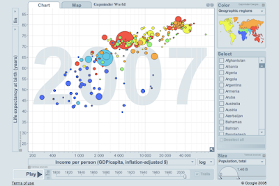
Information graphics is becoming such a hot area. Edward Tufte was just in business week (slides). I want to be a data scientist when I grow up. One potential role mode is Hans Rosling, the swedish professor behind Gapminder. He has talks on economic development and poverty which use their trendalyzer software. That makes me want to acquire the three skills of data geeks, stats, data munging, and visualization.

Sunday, June 21, 2009

Semantic data in life science

When I first saw RDF I said, "Blech!" Well, that's also what I said when I first saw HTML. But, I'm coming around to it. Sure, it's not pretty, but RDF is a graph and graphs are cool. And, we're starting to see more and more that the relational model of data works less well in some situations than it does in transaction processing, while RDF related tools are moving from vaporware to something more practical.

With the web, a new data model is growing up which can be generalized as a graph, where nodes and edges have properties, plus indexes to quickly find sets of nodes in the graph. The web and its search engines are an instance of this pattern. As the web becomes a channel for structured data, it gets more natural to model your data like this, too. Biology has a great tradition of open data and the network is already a workhorse of modern biology. So, why not structure you data that way?

Tim Berners-Lee, in a TED-talk on the blooming of Linked Data, points out the huge untapped potential of integrating the separate data silos distributed all over the web. Because biology was an early adopter of open data, some of its key assets are open, but poorly linked and not very programmable. Maybe the Semantic Web of Life Science will change that particularly in Systems Biology, which demands the integration of diverse types of data.

Clay Shirky criticized the semantic web for its links to AI, and deductive reasoning, asking "What is the Semantic Web good for?" Well, maybe data integration, rather than inference, is the answer.

Hack biology in your garage

One of the beautiful things about computing is that you don't need anyone's permission. You can set yourself up to do real software engineering or computer science so inexpensively that you need no sponsorship from a corporation or academic institution. This is one of the keys to the amazing creativity that's come out of computing in the past few decades. Now, the same effect is showing up in biology. There's a whole DIY movement, described in an article in h+:

Friday, June 05, 2009

Practical semantic web

Toby Segaran, author of the super-fun Programming Collective Intelligence, has a nice talk titled Why Semantics? available about practical semantic web. If you immediately think of jumbo shrimp or military intelligence, you're not alone. But, his talk isn't pie-in-the-sky. He explains some of the contortions commonly used to shoe-horn freeform data into relational databases, then shows that these issues are being addressed using the graph databases that are part of the semantic web effort.

His upcoming book on the subject is Programming the Semantic Web.

He mentions a few good resources:

Sesame - a RDF data store
Exhibit from MIT's Simile project
Linking Open Data
Geonames
Music Brainz
Freebase

Tuesday, June 02, 2009

How to plot a graph in R

Here's a quick tutorial on how to get a nice looking graph out of R (aka the R Project for Statistical Computing). Don't forget that help for any R command can be displayed by typing the question mark followed by the command. For example, to see help on plot, type ?plot.

Let's start with some data from your friends, the Federal Reserve. The fed keeps lots of interesting economic data and they make it pretty easy to get at. What if we're curious about the value of the US Dollar? How's it doing against other major currencies? Let's have a look. I'll use the Nominal Major Currencies Dollar Index. The fed gives us the data here:

http://www.federalreserve.gov/releases/h10/Summary/

First, download the file and load it into your favorite text editor. Replace \s\s+ with \t to create two tab delimited columns. I think this is probably easier than trying to get R to read data separated by at least 2 spaces, as the source file seems to be. Now, load your data into R.

d = read.table('dollar_vs_major_currencies_index.txt', header=F, sep="\t", col.names=c("month", "index"))
dim(d)
[1] 437   2
head(d)
     month    index
1 JAN 1973 108.1883
2 FEB 1973 103.7461
3 MAR 1973 100.0000
4 APRimg 1973 100.8251
5 MAY 1973 100.0602
6 JUN 1973  98.2137

R will show you the structure of an object using the str() command:

str(d)
'data.frame': 437 obs. of  2 variables:
 $ month: Factor w/ 437 levels "APR 1973","APR 1974",..: 147 110 256 1 293 220 184 38 402 366 ...
 $ index: num  108 104 100 101 100 ...

So far so good. R is all about stats, so why not do this?

summary(d$index)
   Min. 1st Qu.  Median    Mean 3rd Qu.    Max. 
  70.32   87.93   95.89   97.48  105.40  143.90

OK, let's get to some plotting. First off, let's try a simple case.

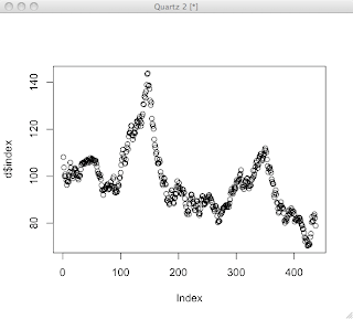
plot(d$index)

That's OK for quickly looking at some data, but doesn't look that great. R can make reasonable guesses, but creating a nice looking plot usually involves a series of commands to draw each feature of the plot and control how it's drawn. I've found that it's usually best to start with a stripped down plot, then gradually add stuff.

Start out bare-bones. All this does is draw the plot line itself.

plot(d$index, axes=F, ylim=c(0,150), typ='l', ann=F)
axes=Fdon't draw axes
ann=Fdon't draw annotations, by which they mean the titles for the plot and the axes
typ='l'draw a line plot
ylimset limits on y axis

Next, let's add the x-axis nicely formatted. We'll use par(tcl=-0.2) to create minor tick marks. The first axis command draws those, but doesn't draw labels. The second axis command draws the major tick marks and labels the years on even decades.

par(tcl= -0.2)
axis(1, at=seq(1, 445, by=12), labels=F, lwd=1, lwd.ticks=1)
par(tcl= -0.5)
axis(1, at=seq(1 + 12*2, 450, by=60), labels=seq(1975,2010,5), lwd=0, lwd.ticks=2)

Note that there's an R package called Hmisc, which might have made these tick marks easier if I had figured it out. Next, we'll be lazy and let R decide how to draw the y-axis.

axis(2)

I like a grid that helps line your eye up with the axes. There's a grid command, which seemed to draw grid lines wherever it felt like. So, I gave up on that and just drew my own lines that matched my major tick marks. The trick here is to pass a sequence in as the argument for v or h (for vertical and horizontal lines). That way, you can draw all the lines with one command. Well, OK, two commands.

abline(v=(12*(seq(2,32,by=5)))+1, col="lightgray", lty="dotted")
abline(h=(seq(0,150,25)), col="lightgray", lty="dotted")

Let's throw some labels on with the title command.

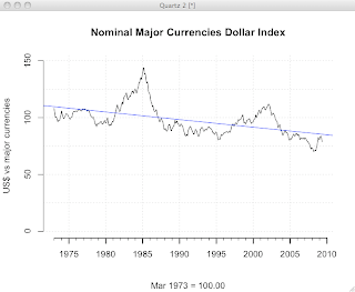
title(main="Nominal Major Currencies Dollar Index", sub="Mar 1973 = 100.00", ylab="US$ vs major currencies")

Finally, let's bust out a linear regression. The lm() function, which fits a linear model to the data, has some truly bizarre syntax using a ~ character. The docs say, "The tilde operator is used to separate the left- and right-hand sides in model formula. Usage: y ~ model." I don't get at all how this is an operator. It seems to mean y is a function of model? ...maybe? In any case, this works. I'm taking it as voodoo.

linear.model = lm(d$index ~ row(d)[,1])
abline(linear.model)

Now, we have a pretty nice looking plot.

The full set of commands is here, for your cutting-and-pasting pleasure.

plot(d$index, axes=F, ylim=c(0,150), typ='l', ann=F)
par(tcl= -0.2)
axis(1, at=seq(1, 445, by=12), labels=F, lwd=1, lwd.ticks=1)
par(tcl= -0.5)
axis(1, at=seq(1 + 12*2, 450, by=60), labels=seq(1975,2010,5), lwd=0, lwd.ticks=2)
par(tcl= -0.5)
axis(2)
abline(v=(12*(seq(2,32,by=5)))+1, col="lightgray", lty="dotted")
abline(h=(seq(0,150,25)), col="lightgray", lty="dotted")
title(main="Nominal Major Currencies Dollar Index", sub="Mar 1973 = 100.00", ylab="US$ vs major currencies")
linear.model = lm(d$index ~ row(d)[,1])
abline(linear.model, col="blue")

...more on R.

Thursday, May 14, 2009

Distributed Annotation System (DAS)

DASDAS is a web based protocol for exchanging genomic annotation data introduced by Lincoln D. Stein, Sean Eddy, and Robin Dowell in a 2001 paper in BMC Bioinformatics. The spec defines URL requests used by clients to query servers and XML documents served up in response. The data model implied by DAS XML is partially an XML-ified version of GFF (another Lincoln Stein project), modified to better fit the hierarchical structure of XML. Simplified, there are sequences, which have a start, stop and description and annotations (aka features). The DAS data type for sequences is designed to help deal with ongoing revisions to genome assemblies. The reference sequence is a hierarchical structure of fragments of genome called segments. Smaller segments of sequence are assembled into larger units such as contigs or whole chromosomes. This makes the annotation data more resilient to revised assembly of the genome, but leaves some of the responsibility of reducing the data to a common basis in the hands of the clients. Annotations have types, methods, and categories. Types correspond to feature type tags from EMBL and GenBank, for example "exon", "CDS" (for coding sequence), or "tRNA". A method is a laboratory procedure or computational method for discovering the feature. Categories seem vaguely defined to me. They list "Homology", "variation" and "transcribed" as examples. Annotations can be filtered by type and/or category. On the off chance that you're writing a genome browser, this might all come in handy. Links:

Wednesday, April 29, 2009

MySQL cheat-sheet

Well, now that MySQL is Oracle's SQL, I dunno how long this information will remain useful. But, here it goes:

Start

If you've installed MySQL by HomeBrew:

mysql.server start

otherwise...

sudo /usr/local/mysql/bin/mysqld_safe
cnt-z, bg

Set root password

mysqladmin -u root -pcurrentpassword password 'newpassword'

Console

mysql -p -u root

Create DB

create database foo;
use foo;

Create User

create user 'bar'@'localhost' identified by 'some_pass';
grant all privileges on foo.* to 'bar'@'localhost';
grant all privileges on foo.* to 'bar'@'localhost' with grant option;

Show Users

select host, user, password from mysql.user;

Shutdown

mysqladmin -p -u root shutdown

Load data from a table

LOAD DATA infile '/temp/myfile.tsv' INTO TABLE my_table IGNORE 1 lines;

You might get ERROR 13 (HY000): Can't get stat of ... caused by permissions. I get around it by giving full permissions to the file and its parent directory. See man stat for more.

Dump and restore data

mysqldump -p -u [user] [dbname] | gzip > [filename]
gunzip < [filename] | mysql -p -u [user] [dbname]

Docs for the mysqladmin tool and other client programs. SQL syntax docs for create table and select, insert, update, and delete.

BTW, where a server isn't needed, I'm starting to like SQLite a lot.