Applying Semantic Web Services to bioinformatics

Applying Semantic Web Services to bioinformatics: Experiences gained, lessons learnt
Phillip Lord, Sean Bechhofer, Mark D. Wilkinson, Gary Schiltz, Damian Gessler, Duncan Hull, Carole Goble, and Lincoln Stein
International Semantic Web Conference, Vol. 3298 (2004), pp. 350-364, doi:10.1007/b102467

Applying Semantic Web Services to bioinformatics is a 2004 paper on Semantic Web Services in context of bioinformatics, based on the experiences of the myGrid and BioMoby projects. The important and worthy goal behind these projects is enabling composition and interoperability of heterogeneous software. Is Semantic Web technology the answer to data integration in biology? I'm a little skeptical.

Here's a biased selection of what the paper has to say:

• "The importance of fully automated service discovery and composition is an open question. It is unclear whether it is either possible or desirable, for all services, in this domain..."
• "Requiring service providers and consumers to re-structure their data in a new formalism for external integration is also inappropriate."
• "Bioinformaticians are just not structuring their data in XML schema, because it provides little value to them."
• "All three projects have accepted that much of the data that they receive will not be structured in a standard way. The obvious corollary of this is that without restructuring, the information will be largely opaque to the service layer."

A couple of interesting asides are addressed:

• Most services or operations can be described in terms in inputs and outputs and configuration parameters or secondary input. When building a pipeline, only main input and output need be considered, leaving parameters for later.
• A mixed a user base divided between biologists and bioinformaticians is one difficulty noted in the paper. I've also found that tricky. Actually, the situation has changed since the article was written. Point-and-click biologists are getting to be an endangered species. The crop of biologists I see coming up these days is very computationally savvy. What I think of as the scripting-enabled biologist is a lot more common. Those not so enabled are increasingly likely to specialize in wet-lab work and do little or no data analysis.

In BioMOBY Successfully Integrates Distributed Heterogeneous Bioinformatics Web Services. The PlaNet Exemplar Case, (2005) Wilkinson writes,

...interoperability in the domain of bioinformatics is, unexpectedly, largely a syntactic rather than a semantic problem. That is to say, interoperability between bioinformatics Web Services can be largely achieved simply by specifying the data structures being passed between the services (syntax) even without rich specification of what those data structures mean (semantics).

In The Life Sciences Semantic Web is Full of Creeps!, (2006) Wilkinson and co-author Benjamin M. Good write, "both sociological and technological barriers are acting to inhibit widespread adoption of SW technologies," and acknowledge the complexity and high curatorial burden.

The Semantic Web for the Life Sciences (SWLS), when realized, will dramatically improve our ability to conduct bioinformatics analyses... The ultimate goal of the SWLS is not to create many separate, non-interacting data warehouses (as we already can), but rather to create a single, ‘crawlable’ and ‘queriable’ web of biological data and knowledge... This vision is currently being delayed by the timid and partial creep of semantic technologies and standards into the resources provided by the life sciences community.

These days, Mark Wilkinson is working on SADI, which “defines an open set of best-practices and conventions, within the spectrum of existing standards, that allow for a high degree of semantic discoverability and interoperability”.

More on the Semantic Web

...looks like this old argument is still playing out.

• The Semantic Web, Tim Berners-Lee, James Hendler and Ora Lassila, 2001
• The Semantic Web, Syllogism, and Worldview, Clay Shirkey, 2003
• A Response to Clay Shirky's “The Semantic Web, Syllogism, and Worldview”, Paul Ford, 2003
• Semantic Web Revisited, 2006
• Kate Ray's mini-documentary Web 3.0
• The Fate of the Semantic Web, a 2010 Pew Research Center survey, summarized by ReadWriteWeb.

Finding the right questions

A 2010 PLOS Biology article, Finding the right questions: exploratory pathway analysis to enhance biological discovery in large datasets, makes some good points about exploratory analysis of noisy biological data and the design of software to help do it.

At a time when biological data are increasingly digital and thus amenable to computationally driven statistical analysis, it is easy to lose sight of the important role of data exploration. Succinctly defined over 30 years ago by John Tukey, exploratory data analysis is an approach to data analysis that focuses on finding the right question, rather than the right answer. In contrast to confirmatory analysis, which involves testing preconceived hypothesis, exploratory data analysis involves a broad investigation, a key component of which may be visual display. Though his arguments predate personal computing and thus focus on graph paper and ink, the point still stands: good data visualization leads to simpler (better) descriptions and underlying fundamental concepts. Today, there is tremendous potential for computational biologists, bioinformaticians, and related software developers to shape and direct scientific discovery by designing data visualization tools that facilitate exploratory analysis and fuel the cycle of ideas and experiments that gets refined into well-formed hypotheses, robust analyses, and confident results.

The authors are involved in Wikipathways, an open platform for curation of biological pathways comparable to KEGG and Ingenuity Pathway Analysis, MetaCyc, and Pathway Commons, and this provides the context for their comments. But, most of their conclusions apply more generally to software for research, where the goal is to enable “researchers to take a flexible, exploratory attitude and facilitate construction of an understandable biological story from complex data.”

...instead of aiming for a single, isolated software package, developers should implement flexible solutions that can be integrated in a larger toolbox [...], in which each tool provides a different perspective on the dataset.

For developers, realizing that exploratory pathway analysis tools might be used not only in isolation but also with other software and different types of data in a flexible analysis setup might guide software design and implementation.

Effective data integration

Flexibility and interactivity are keys to effectiveness. “Determining what to integrate and how to present it to the user depends on the context and the question being asked.” Researchers often need to follow up on a weak or uncertain signal by finding confirmatory evidence in relevant orthogonal or correlated datasets. This emphasizes the importance of well curated data, whether pathways or annotated genome assembies, which can form the scaffolding on which integration takes place.

Providing an API, in addition to UI, opens up possibilities for scripting and automation and enables advanced users to “combine functionalities of different tools to perform novel types of analysis.” The authors note that defining general data models increases reusability and unity among software tools. This resonates with my own experience. One of the key virtues of Gaggle is it's highly general data model consisting of basic data structures - list, matrix, network, table, and tuples - free of specific semantics.

Also noted are the difficulties which make current analysis tools “rather isolated and hard to combine”, specifically:

• reformatting data
• mapping identifiers
• learning curve of multiple software packages

“Succinctly defined over 30 years ago by John Tukey, exploratory data analysis is an approach to data analysis that focuses on finding the right question, rather than the right answer.” We've not yet found the right answer for data integration for biology, but it's clear that “integration of annotations and data is critical to extracting the full potential from large and high-throughput datasets.” This paper contains some exceptionally clear thinking on building software tools that will help bring that about.

Citation

Kelder T, Conklin BR, Evelo CT, Pico AR (2010) Finding the Right Questions: Exploratory Pathway Analysis to Enhance Biological Discovery in Large Datasets. PLoS Biol 8(8): e1000472. doi:10.1371/journal.pbio.1000472

Ingenuity

When I was a little whelp, I had a brief and unsuccessful engagement at a bioinformatics startup in the bay area called Ingenuity. The company had a cool idea, a knowledge base for molecular biology, and smart and creative people to implement it. I was tasked, by a long-haired, Tufte-toting, Stanford grad-student, with developing new and rich UI elements with the budding new technology at the time, dynamic HTML. In particular, I was to implement a search bar that could automatically suggest terms from an ontology - the autocomplete feature.

There was even a prototype that sort-of worked on the right version of Netscape when the server 30 feet away. I pulled my hair out trying to get it working consistently across browsers. A better engineer, say John Resig, might have pulled it off, but I had to admit defeat. Like many DHTML toys of the time, it just wasn't ready for production. So, I recommended scrapping the idea in favor of a simple "google-box". This was not well received and my tenure was not long in coming to a close.

For years after, I'd argue on every project for simple, stripped-down web UIs. "Look at Google," I'd say, pointing to the minimalist search box. Trying to do anything advanced in a browser, I'd warn, was an invitation to cross-browser compatibility issues and nightmarish debugging sessions.

Meanwhile, as if to make me look like a bozo (as if I need any help), Google introduced autocomplete, AKA Google Suggest, first as a Google Labs project, in 2004 and finally rolled out autocomplete on the main Google page in 2008. So much for my "Look at Google" argument. Not that it matters now, but I feel slightly vindicated by the fact that it took even the mighty Google this long to deploy a feature that I was basically shit-canned for failing to implement in 2000. ...not that I'm bitter. But, anyway, back in the present day...

Doug Basset, Chief Scientific Officer at Ingenuity gave a demo last week at the ISB, where I now reside, showing off Ingenuity Variant Analysis, a new tool built on top of their knowledge base that helps find disease-causing genetic variations in resequencing data.

The basic trick is to filter down the millions of genetic variants found in any individual genome to those consistent with a given condition, starting with it's frequency in the population and genetic properties like homo- or heterozygosity. The neat part comes next.

For each variant surviving this far, the program traverses the graph of facts in the knowledge base. Of course, it will find known associations between variants or their host genes and disease. What's better, it can also find relationships a few degrees removed from direct implication. Say, A turns off B with regulates C. The biological process to which C belongs runs amok in disease X. Suddenly, a variant in a functional domain of gene A looks like an interesting candidate. If it works, you end up with a handful of genes with enough evidence to warrant further investigation.

The products's flash-based UI is very slick and modern, with drop-shadows, ghosting and barber-pole progress bars. Tables have spiffy little sparkline graphics. Right in the middle of the demo, a search dialog popped up and there was the autocomplete feature, mocking me. It's certainly no big deal these days. My current project has an autocompleting search box, too, thanks to jQuery and Solr. But, I guess the memory of flubbing that gig still has a little sting left in it.

Twitter feature request

For a long time, I just didn't get Twitter, thinking that nothing of substance could fit in 140 characters. The way I've come to use it is like scanning the headlines on a newspaper, following links to read more about interesting items. I follow folks that are interested in the same nerdy topics I am, in effect like a personal slashdot or hacker news with the riff-raff filtered out, or rather the interesting people filtered in.

Still, my cluster of interests is eclectic and my interests tend to only partially overlap with the people I follow. So, what I want is a feature that will help automatically weed out the stuff I don't care about.

I mostly read tweets on my phone using the Android version of TweetDeck. What if I could swipe right on a tweet for something I like, and swipe left to shit-can a lame tweet? The app could keep track of what I've liked or not and use that as an ever-growing training set to classify new tweets as interesting or dreck. The same data could also be used to find people I should follow or interesting tweets from people I don't necessarily want to follow, etc.

In my case, the app would soon learn to terminate sports-related tweets with deadly efficiency. Also, for you foursquare users, any tweet that starts with "I'm at..." would be ruthlessly eliminated. It would work great for facebook feeds as well, deleting all those "Your sister-in-law just unlocked the Cattywampus badge on whatever-game".

This must already exist. Is this what prismatic is? Maybe, I'll find out if I get my invite!

Update

Looks like I'm not the only one wanted to waste time more efficiently. Seattle hacker Joel Grus built a classifier for Hacker News stories using naive Bayes. Joel gave a nice lightning talk at the latest Seattle Data/Analytics/Machine-Learning MeetUp.

Practical advice for applying machine learning

Sprinkled throughout Andrew Ng's machine learning class is a lot of practical advice for applying machine learning. That's what I'm trying to compile and summarize here. Most of Ng's advice centers around the idea of making decisions in an empirical way, fitting to a data-driven discipline, rather than relying on gut feeling.

Training / validation / test

The key is dividing data into training, cross-validation and test sets. The test set is used only to evaluate performance, not to train parameters or select a model representation. The rationale for this is that training set error is not a good predictor of how well your hypothesis will generalize to new examples. In the course, we saw the cross-validation set used to select degrees of polynomial features and find optimal regularization parameters.

Model representation

The representation of the hypothesis, the function h, defines the space of solutions that your algorithm can find. The example used in the class was modeling house price as a function of size. The model tells you what parameters your algorithm needs to learn. If we've selected a linear function, then there are two parameters, the slope and intersect of the line.

Feature selection and treatment

Are the given features sufficiently informative to make predictions? Asking whether a human expert can confidently predict the output given the input features will give a good indication.

At times, it may be necessary to derive new features. Polynomial features, for example, can let linear regression fit non-linear functions. Computing products, ratios, differences or logarithms may be informative. Creativity comes in here, but remember to test the effectiveness of your new features on the cross-validation set.

Features are on different scales may benefit from feature scaling. Mean normalizing and scaling to a standard deviation of one puts features on an even footing.

Gathering data might be expensive. Another option is artificial data synthesis, either creating new examples out of whole cloth or by transforming existing examples. In text recognition, a library of digital fonts might be used to generate examples, or existing examples might be warped or reflected.

Overfitting

Often, a learning algorithm may fit the training data very well, but perform poorly on new examples. This failure to generalize is called overfitting.

The classic example is fitting a high degree polynomial, which can lead to a very curvy line that closely fits a large number of data points. Our hypothesis is complex and might be fitting noise rather than an underlying relationship and will therefore generalize poorly.

One way to combat this problem is to use a simpler model. This is valid, but might be limiting. Another option is regularization, which penalizes large parameter values. This prioritizes solutions fitting the training data reasonably well without curving around wildly.

Regularization can be tuned by plotting training set error and validation set error as functions of the regularization parameter, lambda.

Tuning the trade off between bias vs variance.

The steps we take to improve performance depend on whether our algorithm is suffering from bias or variance. A learning curve is a diagnostic that can tell which of these situations we're in, by plotting training error and validation error as a function of training set size. Look for high training and cross-validation error indicating high bias or a steadily decreasing validation error, with a gap between validation and training error indicating high variance.

Bias

A high bias model has few parameters and may result in underfitting. Essentially we're trying to fit an overly simplistic hypothesis, for example linear where we should be looking for a higher order polynomial. In a high bias situation, training and cross-validation error are both high and more training data is unlikely to help much.

• find more features
• add polynomial features
• increase parameters (more hidden layer neurons, for example)
• decrease regularization

Variance

Variance is the opposite problem, having lots of parameters, which carries a risk of overfitting. If we are overfitting, the algorithm fits the training set well, but has high cross-validation and testing error. If we see low training set error, with cross-validation error trending downward, then the gap between them might be narrowed by training on more data.

• more training data
• reduce number of features, manually or using a model selection algorithm
• increase regularization

Error analysis

To improve performance of a machine learning algorithm, one helpful step is to manually examine the cases your algorithm gets wrong. Look for systematic trends in the errors. What features would have helped correctly classify these cases?

For multi-step machine learning pipelines, ceiling analysis can help decide where to invest effort to improve performance. The error due to each stage is estimated by substituting labeled data for that stage, revealing how well the whole pipeline would perform if that stage had no error. Stepping through the stages, we note the potential for improvement at each one.

Precision/Recall

It's helpful to have a single number to easily compare performance. Precision and recall and the F1 statistic can help when trying to classify very skewed classes, where one class is rare in the data. Simply taking a percentage of correct classifications can be misleading, since always guessing the more common class means you'll almost always be right.

precision: true positives / predicted positives, predicted positives = true positives + false positives (Of all the patients we predicted to have cancer, what fraction actually has cancer?)

recall: true positives / actual positives, actual positives = true positives + false negatives (Of all the patients that really had cancer, how many did we correctly predict?)

F1 = 2·p·r / (p + r)

Miscellaneous tips

Principle component analysis (PCA) can help by reducing dimensionality of high-dimensional features. Collapsing highly correlated features can help learning algorithms run faster.

Often, incorrectly implemented machine learning algorithms can appear to work, producing no obvious error, but simply converging slower or with more error than a correct implementation. Gradient checking is a technique for checking your work, applied in the class to back propagation, but probably more generally applicable.

The recommended approach

Quickly testing ideas empirically and optimizing developer time is the approach embodied in these steps:

• First, implement a simple quick and dirty algorithm, plot learning curves, and perform error analysis.
• Create a list of potential ideas to try to improve performance. Then, start trying promising ideas, using the validation set to test for improvement.
• Use a learning algorithm with many parameters and many features - low bias. Get a very large training set.

Supporting that last point is the findings of Banko and Brill, 2001.

“It's not who has the best algorithm that wins. It's who has the most data.”

• diagrams by Andrew Ng
• ..more on the machine learning class

SDCube and hybrid data storage

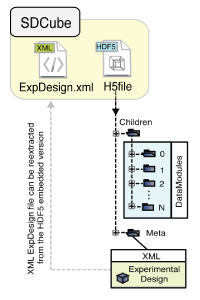
The Sorger lab at Harvard published a piece in the February 2011 Nature Methods that shows some really clear thinking on the topic of designing data storage for biological data. That paper, Adaptive informatics for multifactorial and high-content biological data, Millard et al., introduces a storage system called SDCubes, short for semantically typed data hypercubes, which boils down to HDF5 plus XML. The software is hosted semanticbiology.com.

This two part strategy applies HDF5 to store high-dimensional numeric data efficiently, while storing sufficient metadata in XML to reconstruct the design of the experiment. This is smart, because with modern data acquisition technology, you're often dealing with volumes of data where attention to efficiency is required. But, experimental design, the place where creativity directly intersects with science, is a rapidly moving target. The only hope of capturing that kind of data is a flexible semi-structured representation.

This approach is very reminiscent, if a bit more sophisticated, than something that was tried in the Baliga lab called EMI-ML, which was roughly along the same lines except that the numeric data was stored in tab-separated text files rather than HDF5. Or to put it another way, TSV + XML instead of HDF5 + XML.

Another ISB effort, Addama (Adaptive Data Management) started as a ReSTful API over a content management system and has evolved into a ReSTful service layer providing authentication and search and enabling access to underlying CMS, SQL databases, and data analysis services. Addama has ambitions beyond data management, but shares with SDCube the emphasis on adaptability to the unpredictable requirements inherent in research by enabling software to reflect the design of individual experiments.

There's something to be said for these hybrid approaches. Once you start looking, you see a similar pattern in lots of places.

• NoSQL - SQL hybrids
• SQL - XML hybrids. SQL-Server, for one, has great support for XML enabling XQuery and XPath mixed with SQL.
• Search engines, like Solr, are typically used next to an existing database
• Key/value tables in a database (aka Entity–attribute–value)

Combining structured and semi-structured data allows room for flexibility where you need it, while retaining RDBMS performance where it fits. Using HDF5 adapts the pattern for scientific applications working with vectors and matrices, structures not well served by either relational or hierarchical models. Where does that leave us in biology with our networks?. I don't know whether HDF5 can store graphs. Maybe we need a triple hybrid relational-matrix-graph database.

By the way, HDF5 libraries exist for several languages. SDCube is in Java. MATLAB can read HDF5. There is an HDF5 package for R, but it seems incomplete.

Relational databases work extremely well for some things. But, flexibility has never been their strong point. They've been optimized for 40 years, but shaped by the transaction processing problems they were designed to solve, and they just get awkward for certain uses, to name some - graphs, matrices and frequently changing schemas.

Maybe, before too long the big database vendors go multi-paradigm and we'll see matrices, graphs, key-value pairs, XML and JSON as native data structures that can be sliced and diced and joined at will right along with tables.

More information

• Quantitative data: learning to share, an essay by Monya Baker in Nature Methods, describes how "Adaptive technologies are helping researchers combine and organize experimental results."

Neural Networks

Exercise 4 in Andrew Ng's Machine Learning class is on neural networks. Back in the cretaceous period, in 1994 or so, in one of the periodic phases of popularity for neural networks, I hacked up some neural network code in Borland Turbo C++ on a screaming 90MHz Pentium. That code is probably on a 3 1/2 inch floppy in the bottom of a box somewhere in my basement. Back then, I remember being fascinated by the idea that we could get a computer to learn by example.

Neural networks go in and out of style like miniskirts. [cue lecherous graphic.] Some people scoff. Neural networks are just a special cases of Bayesian networks, they say, and SVMs have more rigorous theory. Fine. But, it's a bit like seeing an old friend to find that neural networks are respectable again.

To see how neural networks work, let's look at how information flows through them, first in the forward direction.

(Andrew Ng)

Forward Propogation

An input example X_t becomes the activation at the first layer, the n x 1 vector a1. Prepending a bias node whose value is always 1, we then multiply by the weight matrix, Theta1. This returns z₂, whose rows are the sum of the products of the input neurons with their respective weights. We pass those sums through the sigmoid function to get the activations of the next layer. Repeating the same procedure for the output layer gives the outputs of the neural network.

Implementing this in Octave, I think, could be fully vectorized to compute all training examples at once, but I did this in a loop over t which indexes a single training example, like this:

a1 = X(t,:)';
z2 = Theta1 * [1; a1];
a2 = sigmoid(z2);
z3 = Theta2 * [1; a2];
a3 = sigmoid(z3);

As in the previous cases of linear and logistic regression, neural networks have a cost function to be minimized by moving in short steps along a gradient.

(Andrew Ng)

Back propagation

The gradients are computed by back propagation, which pushes the error backwards through the hidden layers. It was the publication of this algorithm in Nature in 1986, that led to the resurgence that I caught the tail end of in the 90's.

Cross-validation, regularization and gradient checking

When using neural networks, choices need to be made about architecture, the number of layers and number of units in each layer. Considerations include over-fitting, bias and computational costs. Trying a range of architectures and cross-validating is a good way to make this choice.

The layered approach gives neural networks the ability to fit highly non-linear boundaries, but also makes them prone to over-fitting, so it's helpful to add a regularization term to the cost function that penalizes large weights. Selecting the regularization parameter can be done by cross-validation.

Translating the math into efficient code is tricky and it's not hard to get incorrect implementations that still seem to work. It's a good idea to confirm the correctness of your computations with a technique called gradient checking. You compute the partial derivatives numerically and compare with your implementation.

Back in the day, I implemented back-prop twice. Once in my C++ code and again in Excel to check the results.

A place in the toolbox

The progression of ideas leading up to this point in the course is very cleverly arranged. Linear regression starts you on familiar ground and helps introduce gradient descent. Logistic regression adds the simple step of transforming your inputs through the sigmoidal function. Neural networks then follow naturally. It's just logistic regression in multiple layers.

In spite of their tumultuous history, neural networks can be looked at as just another tool in the machine learning toolbox, with pluses and minus like other tools. The history of the idea is interesting, in terms of seeing inside the sausage factory of science.